
A personal financial dashboard in Google Sheets is one tab that summarizes your other tabs. Six tiles cover what most people want to see: net worth, monthly cash flow, savings rate, total debt and blended rate, goal progress, and investments. Each tile is a few summary formulas (mostly SUMIFS, SUMPRODUCT, and SPARKLINE) pointing at source tabs, laid out to fit on one screen with no scrolling.
A dashboard does one thing. It answers the question “where am I right now” without making you click through three tabs and a chart to find out. Everything else (the transaction log, the asset list, the goal sheets) is the engine room. The dashboard is the gauges.
This guide walks through building one from a blank tab. Six tiles, the formulas behind each, a layout that fits on a 13-inch laptop, and the trade-offs to make if your data does not yet match the assumptions.
What a dashboard is - and what it isn’t
A dashboard is a summary view. It pulls totals from elsewhere and presents them in a layout you can read at a glance. It is not a data-entry surface. The dashboard reads, the other tabs write.
That separation matters because dashboards break when people start editing them. A formula gets overwritten with a hard-coded number, a sort order gets shuffled, and three weeks later the savings rate tile is showing last quarter’s data. Treat the dashboard as read-only by convention. All edits happen on the source tabs.
The other thing a dashboard is not: a chart gallery. Six small charts on one tab is harder to read than six numbers with one trend line. Resist the urge to make everything a graph. Most tiles are a single number plus a tiny indicator of direction.
The six standard tiles
Most personal financial dashboards land on the same six tiles. Different templates relabel or rearrange them, but the underlying questions are stable.
| Tile | Question it answers | Source tab |
|---|---|---|
| Net worth | What am I worth today, and which way is it moving? | Balance sheet |
| Monthly cash flow | Did more come in than went out this month? | Transactions |
| Savings rate | What share of income did I keep? | Transactions or summary |
| Debt | What do I owe, at what blended rate? | Liabilities |
| Goal progress | How close are my top goals to done? | Goals |
| Investments | What is the portfolio worth, and what is allocation? | Holdings |
Some dashboards add a seventh tile - upcoming bills, sinking-fund balances, recent transactions. We argue against that for a first build. Six is already a lot to look at; pushing to seven usually means one of the tiles starts overflowing or gets cropped on smaller screens.
If you do not have data for one of the six tiles yet, leave the tile in place with a “no data yet” placeholder. It is a prompt to set up the source tab, not a reason to delete the tile.
Layout - one screen, no scrolling
The “no scrolling” rule is the single most useful design constraint a personal dashboard has. If you have to scroll to see all the tiles, it is no longer a single view; it is two pages, and the second page gets ignored.
Target viewport: 13-inch laptop, browser zoom at 100 percent, with the Google Sheets toolbar visible. That gives you roughly 24 visible rows and columns A through P at default widths.
A six-tile layout that fits:
+-------------------+-------------------+-------------------+
|   NET WORTH       |  MONTHLY CASH     |  SAVINGS RATE     |
|   $293,900        |  +$1,820          |   18.4%           |
|   (+$3,400 mo)    |  Income $6,400    |   Target 20%      |
|   [12-mo line]    |  Spend $4,580     |   [bar to target] |
+-------------------+-------------------+-------------------+
|   DEBT            |  GOAL PROGRESS    |  INVESTMENTS      |
|   $310,900        |  Emergency 78%    |   $172,600        |
|   Blended 5.4%    |  Down pmt 41%     |   YTD +6.8%       |
|   18-yr payoff    |  Vacation 22%     |   60/30/10 mix    |
+-------------------+-------------------+-------------------+
Three columns, two rows, each tile occupying a 4-column by 8-row block. Headers in row 1 of each tile, the headline number in row 2 at 24pt, the supporting detail beneath at 11pt. Use cell borders to draw tile boundaries; do not use background fills, which fight the conditional formatting later.
Freeze nothing.
Setting up the file
Add a Dashboard tab to an existing personal finance file, or start a new one. If you are building the source tabs from scratch, How to Create an Advanced Personal Finance Tracker in Google Sheets covers the transaction log and category setup that feed most of these tiles. Five source tabs feed it:
Transactions- the running ledger (date, category, merchant, amount)Balance Sheet- assets and liabilities, structured as covered in How to Build a Personal Balance Sheet in Google SheetsGoals- a small table of goal name, target, currentHoldings- investment positions (account, ticker, value, asset class)Net Worth History- month-end net worth snapshots, for the sparkline
Some people merge a few of these (Goals into Balance Sheet, for example). The pattern survives that - the dashboard formulas need to know which tab and which range to point at, and that is all.
Net worth: the headline plus a 12-month line
The headline number is current net worth. The supporting numbers are the change from last month and a 12-month trend line.
Assume Net Worth History has columns A (date, month-end) and B (net worth value), with the most recent row at the bottom.
Current value - the last non-empty value in column B:
=INDEX(B:B, COUNTA(B:B))COUNTA counts non-empty cells, so INDEX(B:B, n) returns row n - the latest entry.
Change vs last month - latest minus previous:
=INDEX(B:B, COUNTA(B:B)) - INDEX(B:B, COUNTA(B:B)-1)Wrap with IFERROR to show ”-” when there is only one month of history:
=IFERROR(INDEX(B:B, COUNTA(B:B)) - INDEX(B:B, COUNTA(B:B)-1), "-")12-month sparkline - the trailing twelve months from the same column:
=SPARKLINE(OFFSET(B1, MAX(0, COUNTA(B:B)-12), 0, MIN(12, COUNTA(B:B)-1), 1), {"charttype","line"; "color","#1f7a4d"; "linewidth", 2})OFFSET carves out the last 12 rows. The MAX(0,...) and MIN(12,...) guard the case where you have fewer than 12 months of history. Sparklines do not label axes; that is the point. They show direction at a glance. The SPARKLINE function reference covers the chart-type and color options if you want to tweak the look.
If the change cell is positive, color it green. If negative, red. Conditional formatting handles that (Google Sheets conditional formatting reference). Format > Conditional formatting > “Format cells if greater than 0” with green text, “less than 0” with red.
Monthly cash flow: in, out, and the gap
Three numbers: income this month, spending this month, the difference.
Assume Transactions has columns A (date), B (category), C (merchant), D (amount), with income entered as positive and expenses as negative. Some templates use a separate column for inflows vs outflows; the formula adjusts trivially.
Income this month:
=SUMIFS(Transactions!D:D, Transactions!D:D, ">0", Transactions!A:A, ">="&EOMONTH(TODAY(),-1)+1, Transactions!A:A, "<="&EOMONTH(TODAY(),0))The date window is “first day of current month through last day of current month”. EOMONTH(TODAY(),-1)+1 is the first of the month; EOMONTH(TODAY(),0) is the last day. The SUMIFS function sums column D only for rows that match every condition, so the same window works on any tab.
Spending this month:
=ABS(SUMIFS(Transactions!D:D, Transactions!D:D, "<0", Transactions!A:A, ">="&EOMONTH(TODAY(),-1)+1, Transactions!A:A, "<="&EOMONTH(TODAY(),0)))ABS() flips the negative sum to a positive number for display.
Cash flow (income minus spending):
=B5 - B6If B5 holds income and B6 holds spending. A positive value means more came in than went out; a negative value means the opposite. Conditional formatting on this cell uses the same green/red pattern as the net worth change.
A note on partial months. Early in the month, the cash flow tile shows the partial total, which can look alarming. Adding a small “(day X of 30)” label next to the headline keeps that in context. The formula:
="Day "&DAY(TODAY())&" of "&DAY(EOMONTH(TODAY(),0))That returns something like “Day 12 of 31” - immediate context for whether the number is mid-stream.
Savings rate against a target
Savings rate is (income minus spending) divided by income. There are stricter definitions (pre-tax vs post-tax, treating debt principal as saving or as spending), and we touch on the trade-offs at the end of this section.
Current month savings rate:
=IFERROR((B5 - B6) / B5, 0)Where B5 is income and B6 is spending from the cash-flow tile above. IFERROR handles divide-by-zero in months where income is 0 (rare, but happens with irregular paychecks).
Format as a percentage: Format > Number > Percent.
Target rate - whatever number you keep separately as your reference. Some people use 20 percent (from the 50/30/20 framework), others use 10 or 30. Hard-code it for now in cell K7:
0.20Format as percent. The 50/30/20 framework is one of several common reference points; high earners in low-cost cities often run higher, parents of young kids often run lower. The number on the dashboard is for context, not for grading.
Progress bar toward target - a sparkline configured as a bar, showing this month’s rate against the target:
=SPARKLINE({MIN(savings_rate, target); MAX(0, target-savings_rate)}, {"charttype","bar"; "color1","#1f7a4d"; "color2","#dddddd"; "max", target})That renders a small horizontal bar showing how much of the target you have hit. When the actual rate exceeds the target, the second segment goes to zero and the bar is fully filled.
On the savings-rate definition: the strict version subtracts taxes, then takes (gross income - taxes - spending) / (gross income - taxes). The loose version uses net pay as the denominator. Both are defensible. Pick one and stay with it; consistency over time is what makes the trend useful.
Total debt, blended rate, and a payoff timeline
Three numbers: total balance, weighted average interest rate, payoff timeline at current payments.
Assume Balance Sheet has a Liabilities section with columns for account, balance, rate, and minimum monthly payment. The minimum payment column makes the payoff calculation honest.
Total debt:
=SUM('Balance Sheet'!Liabilities_Balance)Use a named range or a literal range like 'Balance Sheet'!E2:E20. Named ranges age better when the tab grows.
Weighted average interest rate:
=SUMPRODUCT('Balance Sheet'!Liabilities_Balance, 'Balance Sheet'!Liabilities_Rate) / SUM('Balance Sheet'!Liabilities_Balance)SUMPRODUCT multiplies the two arrays element-wise and sums the result. Dividing by total balance gives the blended rate weighted by how much you owe at each rate. A $200,000 mortgage at 5 percent and a $5,000 credit card at 22 percent come out to about 5.4 percent blended - the mortgage dominates because of the size.
Years to pay off at current minimum payments:
=NPER(weighted_rate/12, -total_min_payment, total_debt) / 12NPER returns the number of months to pay off a loan at a given payment. Dividing by 12 converts to years. The negative sign on payment matches the cash-flow convention used by PMT and FV.
A worked example. Total debt $310,900, blended rate 5.4 percent, total minimums $2,300/month. NPER(0.054/12, -2300, 310900) / 12 returns about 18 years. That is the timeline at minimums only - any extra payment shortens it, sometimes dramatically.
This is the tile where prescriptive language sneaks in most easily. Resist it. The tile shows current trajectory; the reader decides what to do with that.
Goal progress, three at a time
Three goals, each as a percentage with a small progress bar.
Assume Goals has columns A (name), B (target amount), C (current amount), sorted by priority with the top three at the top.
Goal 1 name and percentage:
=Goals!A2
=Goals!C2 / Goals!B2
Format the second as a percent.
Goal 1 progress bar:
=SPARKLINE({Goals!C2, MAX(0, Goals!B2 - Goals!C2)}, {"charttype","bar"; "color1","#1f7a4d"; "color2","#eeeeee"; "max", Goals!B2})That renders a horizontal bar where the filled portion is what you have saved and the unfilled portion is what is left.
Repeat for goals 2 and 3 by pointing at rows 3 and 4 of the Goals tab. The whole tile is six formulas plus three sparklines.
A common question: what counts as a goal? An emergency fund counts. A down payment counts. A vacation fund counts. A vague “I want to save more” does not - it has no number, so the progress bar cannot fill. The article How to Track Multiple Savings Goals in Google Sheets covers the goal-tab structure in more detail.
Investments: portfolio value, YTD return, allocation
Three numbers: total portfolio value, year-to-date return, current asset allocation.
Assume Holdings has columns A (account), B (ticker), C (asset class), D (current value), and a separate Investment History tab with columns A (date) and B (portfolio value) for the YTD calculation.
Total portfolio value:
=SUM(Holdings!D:D)YTD return:
=INDEX('Investment History'!B:B, COUNTA('Investment History'!B:B)) / INDEX('Investment History'!B:B, MATCH(DATE(YEAR(TODAY()),1,1), 'Investment History'!A:A, 1)) - 1That divides the latest portfolio value by the value at the start of the year, minus 1. MATCH(..., 1) finds the row at or before January 1, which handles the case where you do not have an exact January 1 snapshot.
This is a simple total-return number, not money-weighted return. It ignores the timing of contributions. For a portfolio with steady contributions through the year, the gap is small. For a portfolio with one big lump-sum contribution in March, the simple calculation overstates return. XIRR is the honest answer when contributions are uneven; How to Track Investment Returns in Google Sheets walks through the difference.
Asset allocation - three percentages: stocks, bonds, other.
=SUMIF(Holdings!C:C, "Stocks", Holdings!D:D) / SUM(Holdings!D:D)
=SUMIF(Holdings!C:C, "Bonds", Holdings!D:D) / SUM(Holdings!D:D)
=1 - prev_two
Format as percentages. A 60/30/10 mix renders cleanly across one cell line. For a finer breakdown (US equity, international, real estate, cash), the tile gets crowded - five categories is about the limit before the layout starts to suffer.
Conditional formatting for status colors
A dashboard without color cues is harder to read at a glance. A few rules cover most needs:
- Change cells (net worth delta, cash flow): green if positive, red if negative. One rule for each, applied to the cell.
- Savings rate vs target: green if at or above target, amber if within 5 points below, red if more than 5 points below. Three rules on the same cell.
- Goal percentages: a continuous color scale from red (0 percent) to green (100 percent). Format > Conditional formatting > Color scale.
- Blended debt rate: no color - the right rate depends on context (mortgage rates and credit card rates live in different worlds), so a blanket rule misleads.
Resist applying color to the headline numbers themselves. The headline value should read as text; the change indicator gets the color. Otherwise the dashboard becomes a Christmas tree.
The mobile view question
Google Sheets on mobile renders the desktop layout, which means the three-by-two tile grid becomes a side-scrolling experience on a phone. Two options:
- Build a mobile-only tab - a single column of six tiles stacked vertically. Same formulas, different layout. Pin it as the second tab so it is one tap away on mobile.
- Accept the desktop bias - the dashboard is a weekend ritual on a laptop, not a daily check on a phone. This is the more common pattern in practice. The phone is for transaction entry; the laptop is for the summary view.
Some templates do both. Most personal users do not, because maintaining two layouts that have to stay in sync doubles the breakage surface. Pick one.
When the build feels like too much
The dashboard above takes a careful afternoon for someone comfortable with SUMIFS and SPARKLINE. It takes a careful weekend for someone who is not. Both are reasonable investments if you want full control of the structure.
The trade-off is maintenance. Every time a category gets renamed, a goal gets added, or a new investment account opens, the dashboard formulas need a small touch-up. That is fine when you built it and remember why each cell does what it does. It gets painful three months later, when the references no longer match the data and you have to relearn your own file.
For the single-page version that some readers prefer over a tile grid, the companion piece One Page Financial Plan Template walks through a narrative layout - same data, different visualization.
Templates that fit
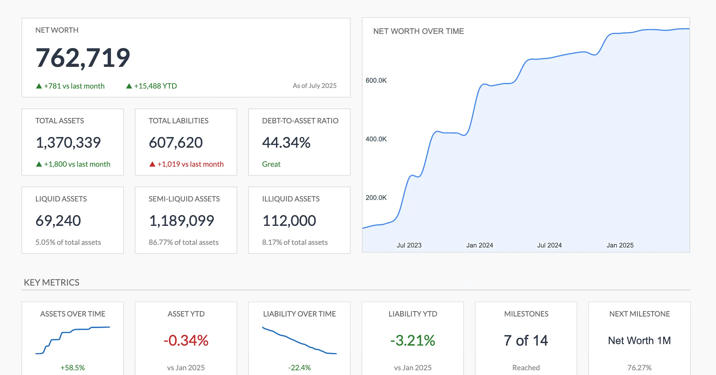
If the net-worth tile is what you actually came for, the Net Worth Tracker ($29) is built around that single question. Its Summary shows net worth with the change against last month and year to date, total assets and total liabilities, a debt-to-asset ratio, assets split into liquid, semi-liquid and illiquid, a net-worth-over-time chart, category breakdowns for both assets and liabilities, and milestone progress. There is no transaction log, cash flow tile or savings rate in it.
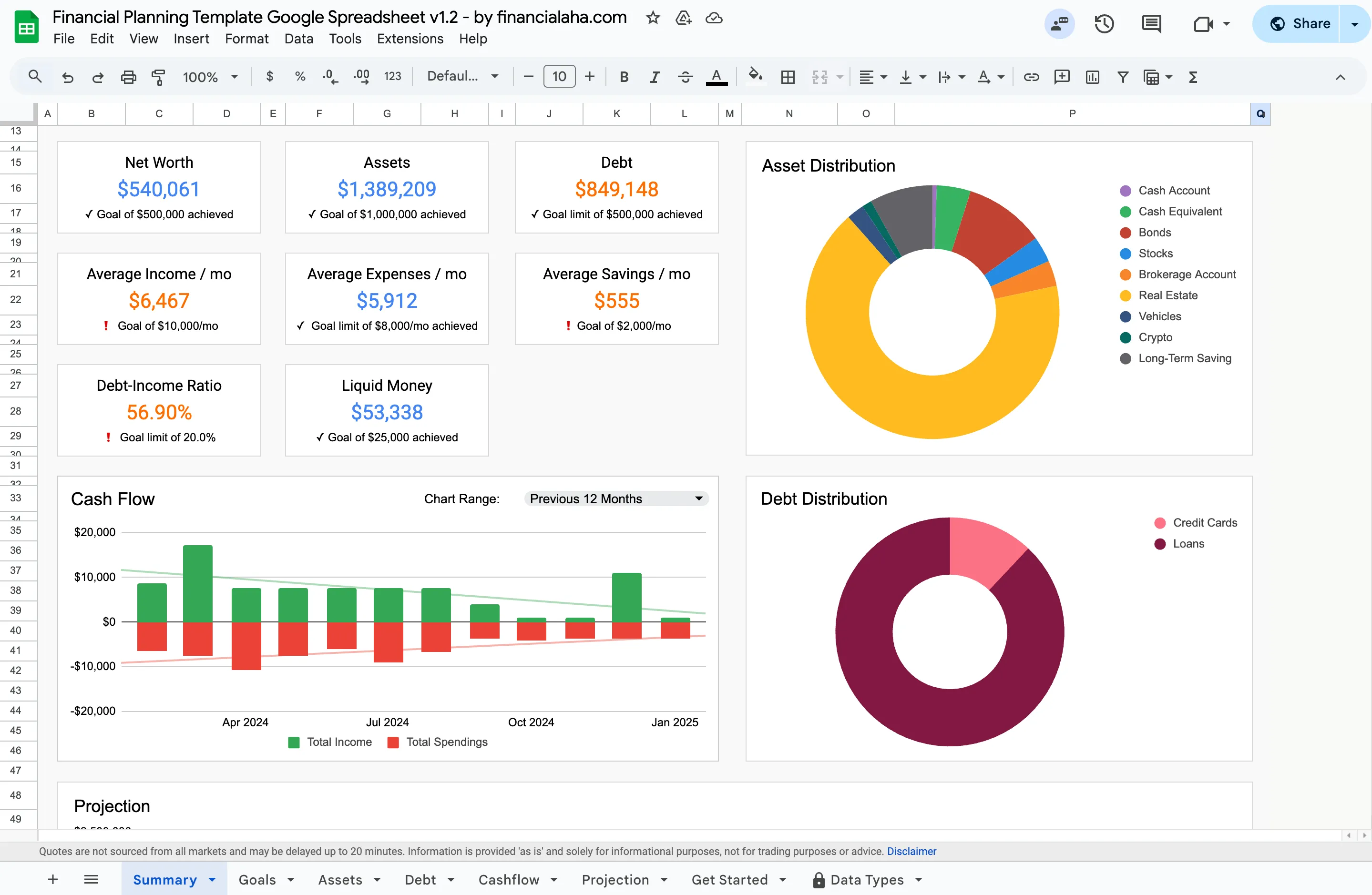
If you want more of the picture on one tab, the Financial Planning Spreadsheet ($29) is the closer match. Its Summary shows net worth, assets, debt, average income, expenses and savings per month, a debt-income ratio, liquid money, a cash flow chart with a range dropdown for All Time Historical, Previous 12 Months or YTD, and asset and debt distribution donuts. A separate Projection tab carries assets, debt and net worth forward month by month to an end year you set. It has no savings-rate tile and no blended-interest-rate tile. Many people start with one and add the other later.
For the keep-building-it-yourself path, the Net Worth Tracker uses the same SPARKLINE calls the tiles above rely on, a line chart for its assets and liabilities trends and a bar chart for milestone progress. Both templates total their tabs with SUM and SUMPRODUCT rather than the SUMIFS date windows above, because neither reads from a transaction log. The longer reference is 15 Essential Google Sheets Formulas for Personal Finance, which walks through XIRR, QUERY, and ARRAYFORMULA as well.
Related
- How to Build a Personal Balance Sheet in Google Sheets - the source-tab structure that feeds the net worth tile.
- 15 Essential Google Sheets Formulas for Personal Finance - the formula reference for
SUMIFS,SPARKLINE,SUMPRODUCT, and the others used above. - One Page Financial Plan Template - the alternative layout when a tile grid feels like too many numbers at once.
Frequently asked questions
Will these dashboard formulas work in Excel too?
Mostly. SUMIFS, SUMPRODUCT, NPER, and EOMONTH behave the same in both. The difference is SPARKLINE: Google Sheets treats it as a cell function, while Excel uses a built-in sparklines feature added from the Insert menu instead, so those in-cell trend lines are set up differently. The layout and the other tiles port over directly.
Do I need a paid Google account for this?
No. Every function used here (SUMIFS, SUMPRODUCT, SPARKLINE, NPER, EOMONTH, conditional formatting) is available in the free version of Google Sheets. No add-ons or Workspace subscription are required.
Do I need to know how to make charts?
Basic charts (SPARKLINE for in-cell trend lines, plus one or two Insert > Chart for larger trends). The article walks through each chart used. No advanced visualization knowledge required.
How does the dashboard get its data?
From other tabs in the same spreadsheet. A 'Net Worth History' tab feeds the net worth tile; a 'Transactions' tab feeds cash flow, and so on. The dashboard is a summary view, not a data-entry view.
Why does the cash flow tile look so low or negative early in the month?
The month-to-date window only counts transactions logged so far, so before payday the tile can show a partial or negative figure. The 'Day X of Y' label in the cash flow section is there to keep that in context. The number fills out as the month's income and spending land.
How often should the dashboard update?
Most of the dashboard updates automatically as the underlying tabs change. Net worth, investment values, and major balances usually update monthly when statements arrive. The dashboard reflects whatever the data shows.
Sources
- SUMIFS function - Google Docs Editors Help
- SPARKLINE function - Google Docs Editors Help
- Use conditional formatting rules in Google Sheets - Google Docs Editors Help
About this article
Formulas written for and checked against Google Sheets function behavior: SUMIFS, SUMPRODUCT, SPARKLINE, NPER, and EOMONTH. Template feature descriptions checked on 2026-09-10 against the shipped Net Worth Tracker Google Sheet (Summary, Assets, Liabilities, Milestones, Setup tabs) and the shipped Financial Planning Spreadsheet (Summary, Goals, Assets, Debt, Cashflow, Projection tabs). Last reviewed September 2026.